FAQ SoilGrids

Q: What is "SoilGrids"

SoilGridsTM (hereafter SoilGrids) is a system for global digital soil mapping that makes use of global soil profile information and covariate data to model the spatial distribution of soil properties across the globe. SoilGrids is a collections of soil pr

Share on:

This page refers to SoilGrids250m version 2.0 : https://soilgrids.org

References:

Common soil chemical and physical properties:

Poggio, L., de Sousa, L. M., Batjes, N. H., Heuvelink, G. B. M., Kempen, B., Ribeiro, E., and Rossiter, D.: SoilGrids 2.0: producing soil information for the globe with quantified spatial uncertainty, SOIL, 7, 217–240, 2021. DOI

Soil water content at different pressure heads:

Turek, M.E., Poggio, L., Batjes, N. H., Armindo, R. A., de Jong van Lier, Q., de Sousa, L.M., Heuvelink, G. B. M. : Global mapping of volumetric water retention at 100, 330 and 15 000 cm suction using the WoSIS database, International Soil and Water Conservation Research, 11-2, 225-239, 2023. DOI

Survey:

We are collecting information on SoilGrids’ user base to improve the products and better understand their uses. Please help us by filling this survey: https://forms.office.com/r/Hmi1GCG7pn

NOTE: We are closing down an old domain "soilgrids.isric.org". Please make sure that you use the current domain "soilgrids.org"

Contents

What is "SoilGrids"?
What do the filename codes mean?
How were the spatial predictions generated?
How were the legends generated?
Which soil properties are predicted by SoilGrids?
Which soil properties will be available in the future?
How were SOC stock maps generated?
What is the SoilGrids data-sharing policy?
How can I access SoilGrids?
How can I use the Homolosine projection?
How can I use SoilGrids in a different projection?
When 100 metre resolution?
SoilGrids at coarser resolution?
Which soil mask map was used?
How is SoilGrids related to the GlobalSoilMap IUSS working group and its specifications?
What happened to the maps of soil types?
What happened to the SoilGrids 2017 layers?
Where is SoilGrids code?
How accurate are the SoilGrids layers?
How can I help improve SoilGrids?
How can SoilGrids help me improve soil maps for my country?
Who provided soil profile data for the SoilGrids effort?
What if I did not find an answer to my question?
Acknowledgements
Cited sources>

What is "SoilGrids"?

SoilGrids^TM (hereafter SoilGrids) is a system for global digital soil mapping that makes use of global soil profile information and covariate data to model the spatial distribution of soil properties across the globe. SoilGrids is a collections of soil property maps for the world produced using machine learning at 250 m resolution. Predictions are made at six standard depths. SoilGrids uses global models that are calibrated using all available input observations and globally available environmental covariates. This results in globally consistent predictions (no abrupt changes in predicted values at country boundaries, etc). SoilGrids spatial predictions (layers) are produced using a reproducible soil mapping workflow, and can therefore be regularly updated as new soil data or covariates become available, after quality control and data standardisation/harmonisation.

SoilGrids maps are a global soil data product generated at ISRIC — World Soil Information as a result of international collaboration. For more technical and scientific information about SoilGrids contact the development team. For more information about ISRIC and collaboration possibilities please contact the ISRIC Director.

SoilGrids250m = set of global maps of soil properties for six depth intervals at 250 m spatial resolution.
SoilGrids = system for global digital soil mapping.
SoilGrids.org = portal to web-services providing access to SoilGrids maps.

What do the filename codes mean?

Each map in SoilGrids has three components:

a master VRT file;
an OVR file with overviews for swift visualisation;
a folder with GeoTIFF tiles.

Each component name is a triplet separated by underscores: property_depthInterval_quantile For instance, the file cfvo_5-15cm_Q05.vrt is the master file for the 5%-quantile prediction of coarse fragments in the 5 cm to 15 cm depth interval. Below each of the components is explained in more detail.

Properties

The table below shows the properties currently mapped with SoilGrids, their description and mapped units. All maps produced with SoilGrids store data as integer values to minimise storage space. Therefore, some properties are provided in units that are not so common in soil science. By dividing the predictions values by the values in the Conversion factor column, the user can obtain the more familiar units in the Conventional units column.

Name	Description	Mapped units	Conversion factor	Conventional units
bdod	Bulk density of the fine earth fraction	cg/cm³	100	kg/dm³
cec	Cation Exchange Capacity of the soil	mmol(c)/kg	10	cmol(c)/kg
cfvo	Volumetric fraction of coarse fragments (> 2 mm)	cm3/dm3 (vol‰)	10	cm3/100cm3 (vol%)
clay	Proportion of clay particles (< 0.002 mm) in the fine earth fraction	g/kg	10	g/100g (%)
nitrogen	Total nitrogen (N)	cg/kg	100	g/kg
phh2o	Soil pH	pHx10	10	pH
sand	Proportion of sand particles (> 0.05 mm) in the fine earth fraction	g/kg	10	g/100g (%)
silt	Proportion of silt particles (≥ 0.002 mm and ≤ 0.05 mm) in the fine earth fraction	g/kg	10	g/100g (%)
soc	Soil organic carbon content in the fine earth fraction	dg/kg	10	g/kg
ocd	Organic carbon density	hg/m³	10	kg/m³
ocs	Organic carbon stocks	t/ha	10	kg/m²

Depth intervals

SoilGrids predictions are made for the six standard depth intervals specified in the GlobalSoilMap IUSS working group and its specifications:

	Interval I	Interval II	Interval III	Interval IV	Interval V	Interval VI
Top depth (cm)	0	5	15	30	60	100
Bottom depth (cm	5	15	30	60	100	200

Prediction quantiles

SoilGrids maps have associated uncertainties as any product derived from a modelling approach. The prediction uncertainty is quantified by probability distributions. For each property and each standard depth interval this distribution is characterised by four parameters:

Q0.05 - 5% quantile;
Q0.50 - median of the distribution;
mean - mean of the distribution;
Q0.95 - 95% quantile.

Uncertainty layer

The additional uncertainty layer displayed at soilgrids.org is the ratio between the inter-quantile range (90% prediction interval width) and the median : (Q0.95-Q0.05)/Q0.50. The values are multiplied by 10 in order to have integers and reduce the size of the datasets.

How were the spatial predictions generated?

SoilGrids uses state-of-the-art statistical methods for digital soil mapping, relying exclusively on open source tools. The models are tailored per soil property and fitted using documented models. For each property, a global model is calibrated using a spatially stratified 10-fold cross-validation procedure. The model produces values at each map location (cell) and standard depth. The prediction distribution is captured in four different maps reporting its 5%, 50% and 95% quantiles, and the mean.

The ‘mean’ and ‘median (0.5 quantile)’ may both be used as predictions of the soil property for a given cell. The mean represents the ‘expected value’ and provides an unbiased prediction of the soil property. The median yields that value for which there is a 50% probability that the true soil property value is greater and a 50% probability that the true value is smaller. For symmetric distributions the mean and median are identical, while the mean is greater than the median for distributions that are skewed to the right (such as soil organic carbon concentration).

The 0.05 and 0.95 quantiles present the lower and upper boundaries of a 90% prediction interval and may be used as a measure of prediction uncertainty following the GlobalSoilMap IUSS working group and its specifications. This interval presents a value range that contains the true soil property value for each cell (which one would measure from a soil sample taken at the centre of the cell) with 90% probability.

Quantiles of the distribution were computed with Quantile Regression Forests (Meinhausen, 2006) as implemented in the ranger package in R. The mean was computed using the default random forests algorithm.

How were the legends generated?

Legends were generated using the natural Breaks algorithm. The legends are available for download in QGIS3 format.

Which soil properties are predicted by SoilGrids?

SoilGrids contains predictions and associated prediction uncertainties for basic soil properties, following the GlobalSoilMap IUSS working group and its specifications: pH (in water), texture fractions, coarse fragments, bulk density, total nitrogen, organic carbon concentration and cation exchange capacity.

Silt size is between 0.002 and 0.050 mm (USDA classification) and between 0.002 and 0.063 mm (ISO and FAO classification). These differences can be registered in WoSIS, but often the required information is absent in the source databases. Presently, no difference is made between the two for the mapping (i.e., reported figures are used independently from the classification used at the source) to avoid the exclusion of a large number of observations.

SoilGrids provides also predictions for 'complex' soil properties such as organic carbon densities at the six standard depths and organic carbon stocks for topsoil (0-30cm) and subsoil (30-100cm, in development). The list of targeted soil properties will be gradually extended, based on user requests and the availability of soil observations.

Which soil properties will be available in the future?

The list of targeted soil properties will be gradually extended, based on user requests and the availability of soil observations. For example we are developing new predictions for texture classes, soil depth and soil hydrological properties. We are also working on maps for subsoil carbon stocks (30-100cm and 100-200cm).

How were SOC stock maps generated?

SOC stock maps (0 to 30 cm) were generated by first calculating the carbon stocks at sampling locations and then calibrating a model to obtain the global map. To calculate carbon stocks, first we modelled the carbon density from SOC concentration, bulk density and proportion of coarse fragments for each observation. Then, the weighted sum of the carbon densities for the observations between 0 and 30 cm was calculated. Finally, a Quantile Random Forest model was calibrated and used for the global map.

The organic layers on top of mineral soils were removed from the calculations and models. The total global carbon stocks obtained with version 2 (599 Pg of carbon for 0 to 30cm) are more in line with other global estimates (see for example: Jackson et al, 2017, Table 2 and Scharlemann et al, 2014).

Are there differences between the soil organic carbon stocks in the latest and former versions of SoilGrids?

There are differences in the calculated stocks between the two versions of SoilGrids. These differences are due to different modelling approaches and different input data.

The SOC stocks in SoilGrids version 2.0 were obtained with a calculate first interpolate later approach. See this page ( How were SOC stock maps generated ) for more details. The SOC stocks in SoilGrids version 2017 were obtained with a interpolate first calculate later approach, where the stocks were calculated from the maps of the input properties (Hengl et al, 2017)

What is the SoilGrids data-sharing policy?

Since 2019, SoilGrids products are provided under the CC BY 4.0 (publicly accessible environmental data; see also the ISRIC software and data policy). SoilGrids contributes to other public global soil data projects. For a review of global soil mapping initiatives and data sets see: Grunwald et al. 2011, Omuto et al. 2013 and Arrouays et al. 2017.

How can I access SoilGrids?

The latest SoilGrids release can be accessed through the following services:

WMS: access for visualisation and data overview. Instructions for using WMS with commonly used GIS software can be found here
WCS: best way to obtain a subset of a map and use SoilGrids as input to other modelling pipelines. Examples on how to access WCS can be found here. In particular, Jupyter notebooks for python and examples with R
WebDAV: download the complete global map(s) in VRT format. We provide examples to access the data from a file browser and programmatically from R, python and Linux bash. Each map has three elements:
- a master VRT file;

- an OVR file with overviews for faster visualisation;

- a folder with the GeoTIFF tiles.

For example, to download the 0.05-quantile prediction of coarse fragments in the 5 cm to 15 cm depth interval the user has to get the files `cfvo_5-15cm_Q05.vrt` and `cfvo_5-15cm_Q05.ovr` and the `cfvo_5-15cm_Q05` folder.

Each map is about 5 GB. All the maps for a single property, with six standard depth intervals and four quantiles per depth occupies about 120 GB.
A new web mapping platform, with a download option, is available at SoilGrids.org.
SoilGrids predictions are been made available on Google Earth Engine as community contributed datasets. Please see here for more details.

How can I use the Homolosine projection?

To deal with an increasing number of inputs and computation demands, SoilGrids has since 2019 been computed on an equal-area projection. After a thorough comparison, the Homolosine projection was identified as the most efficient in an open source software framework (de Sousa et al. 2019). This projection is fully supported by the PROJ and GDAL libraries; therefore, it can be used with any GIS software.

The Homolosine projection is now included in the PROJ database with the code ESRI:54052.

The actual Spatial Reference System (SRS) of the SoilGrids maps is composed by the Homolosine projection applied to the WGS84 datum. This SRS can be added to the PROJ database (the file named epsg) with the following string:

# ISRIC - Homolosine <152160> +proj=igh +datum=WGS84 +no_defs +towgs84=0,0,0 <>

The verbose Well Known Text (WKT) version of this SRS is:




PROJCS["Homolosine", 
    GEOGCS["WGS 84", 
        DATUM["WGS_1984", 
            SPHEROID["WGS 84",6378137,298.257223563, 
                AUTHORITY["EPSG","7030"]], 
   AUTHORITY["EPSG","6326"]], 
        PRIMEM["Greenwich",0, 
            AUTHORITY["EPSG","8901"]], 
        UNIT["degree",0.0174532925199433, 
            AUTHORITY["EPSG","9122"]], 
        AUTHORITY["EPSG","4326"]], 
    PROJECTION["Interrupted_Goode_Homolosine"], 
    UNIT["Meter",1]]

The European Petroleum Survey Group (EPSG) never issued a code for this projection. However, some programmes like MapServer require any SRS to be associated with such a code. For that reason a pseudo EPSG code was created to refer to the SoilGrids SRS: EPSG:152160.

How can I use SoilGrids in a different projection?

The Homolosine projection is not mandatory in any way. The WMS and WCS publish the SoilGrids maps in the following alternative SRSs:

EPSG:4326 - the popular Marinus of Tyre projection (aka Plate Carré) applied on the WGS84 datum. It expands the surface area of the globe by 60%.
EPSG:54009 - Mollweide projection (aka Homolographic) applied to the WGS84 datum (pseudo EPSG code issued by ESRI).
EPSG:54012 - Eckert IV projection applied to the WGS84 datum (pseudo EPSG code issued by ESRI).

The VRT-mosaics can themselves be easily reprojected using the gdalwarp tool. Considering the size of each mosaic, it is best to require a VRT also as output. For example:

gdalwarp -t_srs EPSG:3035 -of VRT ./sand_60-100cm_Q0.5.vrt ./sand_60-100cm_Q0.5_3035.vrt

when can 100m resolution be expected?

Producing global soil information requires extensive infrastructure and resources. ISRIC has so far delivered complete and consistent global soil information products at 1 km and 250 m resolution. SoilGrids1km and SoilGrids250m are a step towards 100 m global soil property maps. The GlobalSoilMap IUSS working group aims at delivering maps at a finer target resolution of 100 m, and various countries have already done so. It is also on the agenda of the SoilGrids team.

SoilGrids at coarser resolution?

Aggregated SoilGrids products are available at a resolution of 1000 m and 5000 m. For this, the mean predictions from the 250 m products were aggregated at the corresponding coarser resolution. The data are available as COG (geotiff, here) from WebDAV (for instructions see here). We are working to produce modelling uncertainty at coarser resolution as well.

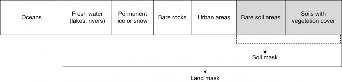
Which soil mask map was used?

The soil mask map provides an approximation of global coverage of soils, i.e. where soil occurs. For the current SoilGrids release, the global soil mask map was derived from the latest ESA land cover map, with the classes Urban (code 190), inland water (code 210), glacier (code 220) and bare surface (code 200) masked out. Predictions have been produced only for soils with vegetation cover and soils without vegetation cover. No estimate is provided for permanent ice areas since they are subject to extreme climatic conditions. The areas that have been masked out are often under-represented in soil surveys, making it difficult to fit a reliable statistical model.

The global soil mask map was derived from the 2015 ESA land cover map.

How is SoilGrids related to the GlobalSoilMap IUSS working group and its specifications?

SoilGrids aims to follow closely the GlobalSoilMap specifications. It focuses exclusively on global predictions, currently with 250 m being the finest resolution.

What happened to the maps of soil types?

SoilGrids version 2.0 includes soil classification maps. These maps are not the result of new predictions, as with soil properties. They are an aggregation of the predictions of the previous release (2017, Hengl et al.).

SoilGrids version 2.0 serves only the Reference Soil Groups (RSG) of the World Reference Base for Soil Resources (WRB 2006), without differentiation by qualifier, in response to the feedback received from users. A single map is now created for each individual RSG. Each map shows the estimated probability of occurrence of the respective RSG within the map cell. This was obtained by summing the probabilities for each map predicted in 2017 that can be associated to the considered RSG for each map cell. Maps of probability occurrence for thirty different RSGs are available. Anthrosols, Technosols and Retisols are not considered, as they were not part of the predictions in SoilGrids version 2017.

An additional, ‘summary’ map provides for each cell the RSG’s with highest probability of occurrence. It is called Most Probable and was obtained by selecting the RSG with the highest probability of occurrence for each map cell from the aggregated RSG probability maps described above. The RAT (Raster Attribute Table) with the legend of the classes is available in the VRT file and here.

A new methodology is currently under development towards a unified soil classification map of the world, that would be more accurate and easier to use. However, the lack of reliable soil class observations remains an important issue. If you have access to such data, please consider contributing and help making a global soil classes map.

We are not working on new USDA soil Taxonomy classes as only a limited number of observations have the necessary USDA soil Taxonomy classification

What happened to the SoilGrids 2017 layers??

For information about the previous version of SoilGrids (2017) , please refer to this page. The 2017 version is no longer actively supported; we only provide a minimum amount of support, mainly related to accessibility of the files.

Where is SoilGrids code?

The code used to generate SoilGrids will be released (under GPL3 license) together with the submission of a journal article describing the methodology and the main results.

How accurate are the SoilGrids layers?

The accuracy of SoilGrids layers is still limited and the variation explained by the models is between 30% and 70%. This is due to many factors:

Limitations on input data spatial distribution and representativeness for different soil types and ecoregions. Certain regions have a very low density of soil profile observations. This is especially relevant for Central Asia, the Artic regions, coastal areas and deserts. We are continuously working on increasing the number and spatial coverage of input data.
Covariates: the covariates used span many soil forming factors. However, we are still missing reliable fine resolution proxies for some important factors, in particular parent material. We are working on extending the set of covariates to improve prediction accuracy.
Modelling choices: Random Forest is a reliable and efficient modelling choice. Other approaches may provide more accurate results at the expenses of heavier computations.

In the current release, we quantified prediction uncertainty as 5th and 95th percentiles. These prediction intervals provide spatially explicit information about the accuracy of the maps.

The issue of accuracy is especially relevant for carbon stocks as these are the results of a complex workflow where numerous sources of uncertainties are combined. For example, the current version has lower than expected values for some organic soils. This is being addressed and investigated.

SoilGrids works on a “rolling release” system; we are providing updates and fixes as soon as these become available. Soon web pages with cross-validation results for all soil properties will be made available.

How can I help improve SoilGrids?

To improve predictions for your country or region, consider contributing/sharing soil profile data to the ISRIC WoSIS database so that your point data can be also used to generate improved predictions. Note that ISRIC will always respect the data policy of the data provider and will not publically share any data unless written permission is given to us to do so. Agencies that contribute data will be acknowledged and listed as a contributing organization on the main SoilGrids portal.

How can SoilGrids help me improve soil maps for my country?

For specific regions, SoilGrids predictions can be used as a covariate to improve prediction of soil properties through a digital soil mapping approach. Predictions for an area of interest can be obtained from the SoilGrids WCS and overlaid with point data. The SoilGrids maps can thus be used as covariates to predict or adjust the values of target variables locally, together with locally available covariates not used by SoilGrids. An example of how a regional scale prediction can be conducted is described in Hengl et al. (2015).

The SoilGrids framework is intended to facilitate global soil data initiatives and to serve as a bridge between global and local soil mapping. Contact ISRIC to explore how we may collaborate to generate or update predictions for your area of interest.

Suggested uses of SoilGrids by national and regional agencies include:

use as a covariate layer for regional mapping;
filling gaps in country-based (bottom-up) global soil information services such as, for instance, developed by the Global Soil Partnership.
providing input soil data for nationally determined contributions (NDC's), such as for instance required by the UNFCCC.

Who provided soil profile data for the SoilGrids effort?

SoilGrids draws on a large collection of geo-referenced soil profile data for the world that are managed in WoSIS (World Soil Information Service; Batjes et al. (2019). Populating WoSIS has been made possible thanks to the contributions and shared knowledge of a steadily growing number of data providers; we gratefully acknowledge their contributions.

What if I did not find an answer to my question?

If you have a technical question about SoilGrids that is not answered in this FAQ, please post it to GIS.StackExchange, under the tag soilgrids. ISRIC staff are subscribed to this tag and will be automatically notified of any new question arising. GIS.StackExchange makes it easier for other SoilGrids users to find quality answers to their questions.

GIS.StackExchange is not a message board or a discussion forum, but a platform for technical questions. If you never used the website before, please take the tour describing the basic functionalities. Please, start by searching the website for similar questions to avoid replicates. If you need to submit a new question please follow the website rules.

Acknowledgements

SoilGrids was funded from ISRIC's core funding, with additional support from the EU-H2020 CIRCASA project.

A wide range of agencies and experts have provided data for the WoSIS/SoilGrids effort; we gratefully thank them for their contributions.

Cited sources

Batjes N.H., Ribeiro E, and van Oostrum Ad (2019). Standardised soil profile data to support global mapping and modelling (WoSIS snapshot 2019). Earth System Science Data Discuss. doi:10.5194/essd-2019-164
Grunwald, S., Thompson, J. A., & Boettinger, J. L. (2011). Digital soil mapping and modeling at continental scales: Finding solutions for global issues. Soil Science Society of America Journal, 75(4), 1201-1213. doi:10.2136/sssaj2011.0025
Hengl T, de Jesus JM, MacMillan RA, Batjes NH, Heuvelink GBM, et al. (2014) SoilGrids1km — Global Soil Information Based on Automated Mapping. PLoS ONE 9(8): e105992. doi:10.1371/journal.pone.0105992
Hengl T, Heuvelink GBM, Kempen B, Leenaars JGB, Walsh MG, Shepherd KD, et al. (2015) Mapping Soil Properties of Africa at 250 m Resolution: Random Forests Significantly Improve Current Predictions. PLoS ONE 10(6): e0125814. doi:10.1371/journal.pone.0125814
Meinshausen, N. (2006). Quantile regression forests. Journal of Machine Learning Research, 7(Jun), 983-999.
Omuto, C., Nachtergaele, F., and Vargas Rojas, R. (2012). State of the Art Report on Global and Regional Soil Information: Where are we? Where to go? Global Soil Partnership technical report. FAO, Rome.
de Sousa, L.M., Poggio, L., Kempen, B.: Comparison of FOSS4G Supported Equal- Area Projections Using Discrete Distortion Indicatrices. ISPRS International Jour- nal of Geo-Information 8(8), 351 (2019) doi:10.3390/ijgi8080351
Jackson, R.B, Lajtha, K, Crow, S.E., Hugelius, G., Kramer, M.G., Piñeiro, G. (2017). The Ecology of Soil Carbon: Pools, Vulnerabilities, and Biotic and Abiotic Controls. Annual Review of Ecology, Evolution, and Systematics, 48:1, 419-445
Scharlemann, JPW, Tanner, EVJ, Hiederer, R., and Kapos, V. (2014) Global soil carbon: understanding and managing the largest terrestrial carbon pool, Carbon Management, 5:1, 81-91

Contact:

SoilGrids team